Polynomial interpolation

A painting of polynomial functions by DALL-E

Connect the dots

How do you get a straight line through two points? You could just represent the line, or line segment, between points $A$ and $B$ by the pair $(A, B)$, which can be ordered or unordered based on whether you care about the direction or not. This abstracts away the geometry and only retains the connectedness. So this is the way it would be represented in topology or in graphs, as it is agnostic to the path taken between the points. It is a non-parametric approach which can be thought of as having omitted information about the travel time.

But what if we want to find the points on the path between the two points? We could design a function, $g$, that can answer whether a given point is on the path or not. The function $g(X) = 0$ if we are on the path, and nonzero otherwise. For example, let’s say we represent the points by vectors in a normed vector space. Then we can use the function

\[g(X) = ||X - A|| + ||X - B|| - ||B - A||\]

This function makes use of the triangle identity, and is equal to zero when the three points $X$, $A$ and $B$ are collinear. Therefore the function indicates whether a point is on the straight line that goes through $A$ and $B$. If we also want to indicate whether $X$ is on the line segment between the points, and not outside, we must also require that

\[||X - A|| \le ||B - A||\]

and

\[||X - B|| \le ||B - A||\]

If we have a dot product then we could also have used it to find the projection $p(X)$ and rejection $r(X)$ of the point $X$ to and from the line, where

\[p(X) = \frac{(X - A) \cdot (B - A)}{(B - A) \cdot (B - A)} (B - A) + A\]

and

\[r(X) = X - p(X)\]

These are vector valued functions, and a function $g$ that satisfies out requirements can then be defined as

\[g(X) = ||r(X)||\]

Parametric lines and curves

The previous examples were abstract topological, and implicit non-parametric, respectively. We can also represent the line using an explicit parametric approach. In this case, we can define a function that takes a parameter $t$, which is often conceptualized as the travel time, and gives an explicit point on the line. We can identify this point $X$ as a function of $t$ with

\[X(t) = (B - A) t + A\]

This function returns $A$ when $t = 0$, $B$ when $t = 1$ and some point in the line segment when $t$ is in the interval $[0, 1]$. With some reordering, using the distributive property, we can alternatively write it as

\[X(t) = (1 - t)A + tB\]

Which can be interpreted as a fade out of $A$ and a fade in of $B$ as $t$ moves from $0$ to $1$. This interpolation between $A$ and $B$ could also be represented by a different parameterization, e.g.

\[X(s) = (1 - s)B + sA\]

where the order of $A$ and $B$ is reversed. Here, the associated parameter values of are changed, but the image of the function is unchanged. The parametrizations are related by $s = 1 - t$. Other parametrizations can be given by scaling and translating $t$.

Linear and affine

The function $X(t)$ is a line through $A$ and $B$ and is often referred to as linear interpolation, or lerp for short, especially in computer graphics and animation fields. The function itself is technically not linear, but affine because of the constant term in the expression. For real valued functions this is the same as the difference between $f(x) = ax$ and $f(x) = ax + b$, where the former function is linear and the latter function is affine. Linear functions are special cases of affine functions with the constant term set to zero, while affine functions can be represented as linear function in one extra variable, say $y$ with the additional constraint that the variables sum to one. e.g.

\[f(x) = ax + by\]

and

\[x + y = 1\]

so that we can solve for $y$ to find that $y = 1 - x$ and retrieve the familiar form of the affine function

\[f(x) = ax + b(1-x)\]

The same is also true for vector valued linear and affine functions, and analogously for multilinear and multiaffine functions.

More points

If we want to parametrically interpolate more than two points, we can no longer use just one line, unless the points happen to be colinear. We can either break the interpolating function into linear pieces, giving a piecewise defined function consisting of line segments between each pair of neighbouring points in the sequence, or, we can interpolate the points by a curve. The curve can be made out of various classes of functions, for example polynomials, rational functions, or trigonometric functions. Each approach have advantages and disadvantages. Combining the piecewise approach with smooth functions gives rise to various spline techniques, most commonly polynomial splines.

Polynomial interpolation

In order for a polynomial function to interpolate a set of points, the polynomial must in general be of degree one less than the number of points we wish to interpolate. E.g linear (degree one) to interpolate two points, and cubic (degree three) to interpolate four points. Keep in mind that in degenerate cases, the interpolating polynomial has lower degree than the number of points. For example if all points coincide, then the interpolating polynomial is just a constant. If they are colinear, then the polynomial is degree one, and if they all lie on a parabola, then the polynomial is quadratic. But we can always interpolate $N$ points with a degree $d = N-1$ polynomial if we include the lower degree polynomials as special cases of the degree $d$ polynomials.

Polynomials can be represented in various different bases, as linear combinations of basis polynomials, but in general the interpolating polynomials of a set of points is unique. The various interpolating polynomials are just the same polynomial expressed in different bases, e.g. Lagrange interpolation, Newton interpolation, etc.

So how can we construct these polynomials? Let’s try to find a set of suitable basis polynomials such that finding the coefficients of the polynomial interpolating the points becomes easy.

A polynomial $p(x)$ is said to interpolate points $y_i$ at $x_i$ if $p(x_i) = y_i$ for all $i$. If we have a set of basis polynomials $\ell_i(x)$ defined in such a way that $\ell_i(x_i) = 1$ and $\ell_i(x_j) = 0$ for all $i \neq j$, then finding the coefficients would be easy, since we could simply set the coefficient of $\ell_i$ to $y_i$ while all other basis functions would be zero at $x_i$ by definition, and thereby canceling all other terms in the polynomials. They would therefore not change the value of $p(x)$ in that position, and we would get that $p(x_i) = y_i$, as required.

Now, how do we come up with such basis functions? Let’s start with considering polynomials on the form

\[\ell(x) = (x - x_0)(x - x_1) \ldots (x - x_n)\]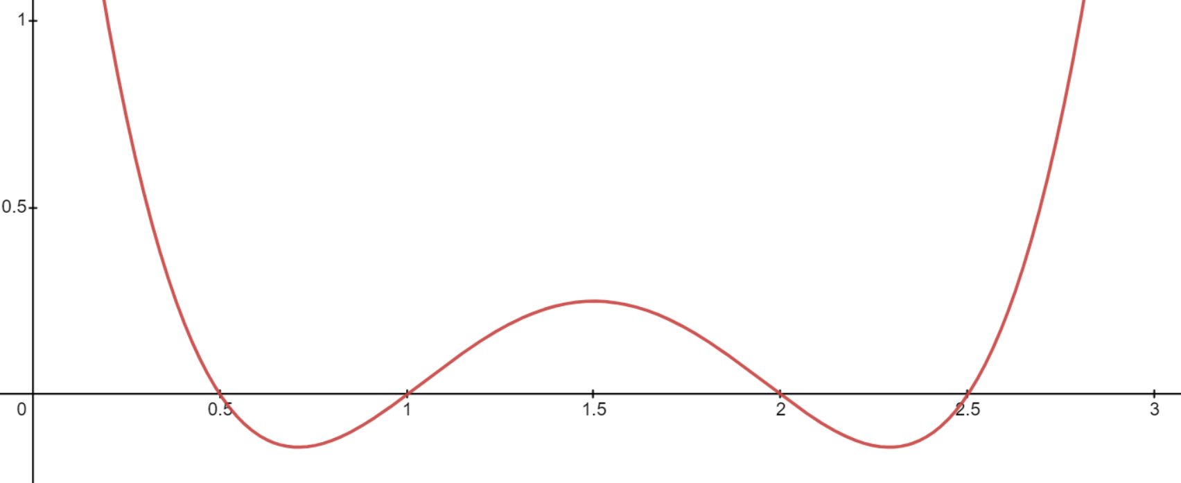

A plot of the function $\left(x\ -\frac{1}{2}\right)\left(x-1\right)\left(x-2\right)\left(x-\frac{5}{2}\right)$

It is clear that $\ell(x)$ is zero at $x = x_i$ for all $i = 1 \ldots n$, since one of the factors in the product would be zero, and thereby making the entire expression zero. Another property of this polynomial is that it is nonzero everywhere else, there are no other roots of the polynomial.

So now we have found a polynomial that is zero on all the given points, so now we need to find a way to make the polynomial be non-zero on one of them. Again, this is easy since we can simply omit that factor from the product. Let’s say we want the polynomial to be nonzero at $x_i$, then we just omit the $(x - x_i)$ factor to get

\[\ell(x) = (x - x_0) \ldots (x - x_{i-1}) (x - x_{i+1}) \ldots (x - x_d)\]

So far so good, but we have not yet found the desired basis polynomials. We didn’t just require that the basis polynomials $\ell_i$ were non-zero at $x_i$ but that they should be equal to one at that point. The fix for this is also straightforward, we must find an expression for the value of the previous polynomial at $x_i$ and divide by that value to get one. For any $\ell_i$ we can find the value by simply evaluating $\ell$ at $x_i$ to get

\[\ell(x_i) = (x_i - x_0) \ldots (x_i - x_{i-1}) (x_i - x_{i+1}) \ldots (x_i - x_d)\]

Since this is just a scaling factor, the polynomial will still have the prescribed roots at $x_j$ for $i \neq j$, and we get the final form

\[\ell_i(x) = \frac{(x - x_0) \ldots (x - x_{i-1}) (x - x_{i+1}) \ldots (x - x_d)}{(x_i - x_0) \ldots (x_i - x_{i-1}) (x_i - x_{i+1}) \ldots (x_i - x_d)}\]

or in product notation

\[\ell_i(x) = \prod_{\substack{j=0\\ j \neq i}}^{d} \frac{(x - x_j)}{(x_i - x_j)}\]

These basis polynomials are called the Lagrange basis polynomials

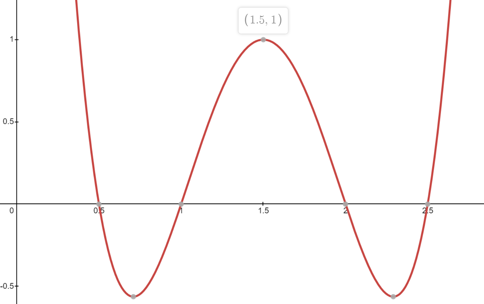
A plot of the function $\ell_2(x) = \frac{\left(x\ -\frac{1}{2}\right)\left(x-1\right)\left(x-2\right)\left(x-\frac{5}{2}\right)}{\left(\frac{3}{2}\ -\frac{1}{2}\right)\left(\frac{3}{2}-1\right)\left(\frac{3}{2}-2\right)\left(\frac{3}{2}-\frac{5}{2}\right)}$

for the node sequence $x_0 = \frac{1}{2}$, $x_1 = 1$, $x_2 = \frac{3}{2}$, $x_3 = 2$ and $x_4 = \frac{5}{2}$

The final interpolating polynomial can then be expressed as simply

\[p(x) = \sum_{i = 0}^d y_i \ell_i(x)\]